Memory is the treasury and guardian of all things.

— Cicero

Introduction

Many programmers are familiar with how the CPU works – or at least in enough details to do their job. This post will build from this understanding to explain some of the important pillars of GPU programming, including roofline charts, threads, memory loads, and the memory hierarchy itself.

High Level Considerations

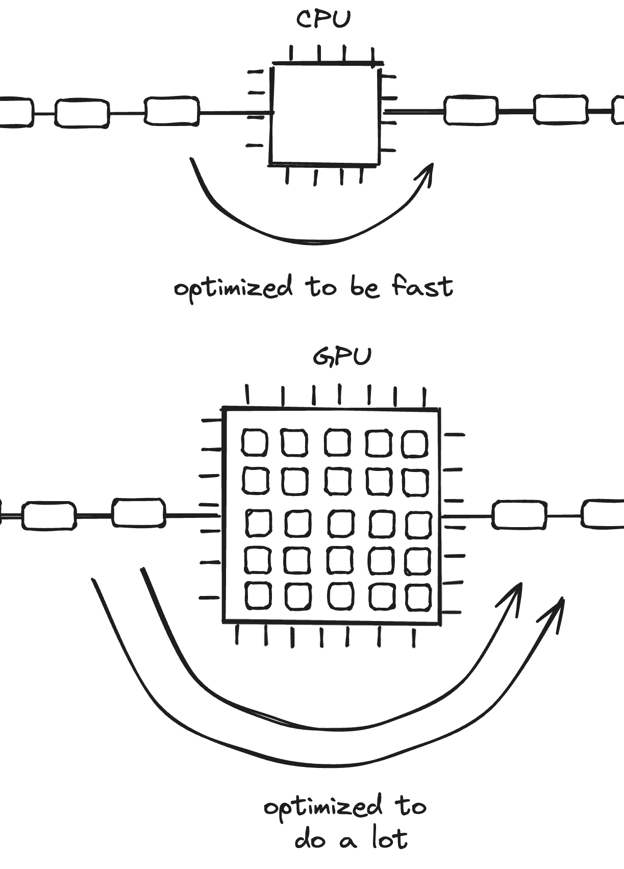
A single CPU core executes instructions sequentially. Computers with a single CPU core can appear to be doing multiple things at the same time, but they’re actually quickly switching between tasks. Because a core can execute only one thread of execution at a time, they’re designed to be fast.

In comparison, GPUs are focused on large workloads that can take more time to complete. The speed of GPUs depends on two primary factors:

• the memory bandwidth, which dictates how long we wait for data to come into the memory,
• the floating-point operations per second, which dictates how fast we can perform operations on that data once it’s there.

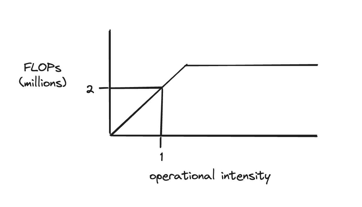
When writing a GPU program, it can be helpful to take these two parameters into account to get the theoretical upper bound of the algorithm we’re writing. We can do this on a roofline chart, which looks like this:

In this graph, the highest FLOPs a specific algorithm can get is plotted on the vertical axis. On the horizontal axis is a new term - operational intensity - which is how many floating-point operations are done per floating-point loaded in.

The shape of the roofline chart is triangular at the beginning, because at low operational intensities, we’re mostly waiting for data to be loaded in. As the operational intensity increases, we become compute-bound, and so the FLOPs cap out.

This helps illuminate a fundamental trade-off. When an algorithm hits our theoretical bounds, we can either (a) do more work per number or (b) load in more numbers per work done. Most programs can be written in multiple forms, and we can use this graph to get hints about the theoretically highest-performing option.¹

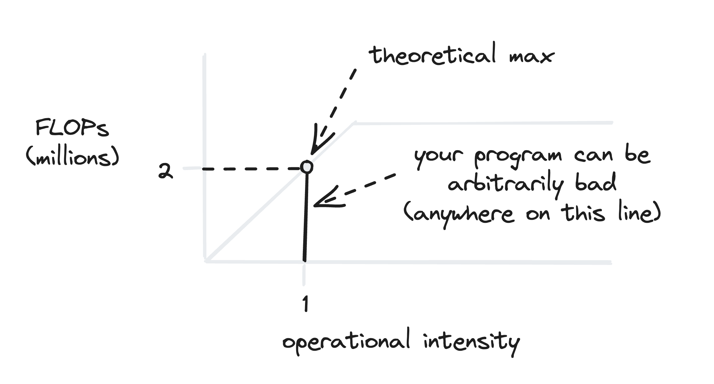
Let’s look at an algorithm which sums up a list of numbers. It has to load in one number per operation (because it has to sum the number it just loaded in) and so the operational intensity is 1.

We can look at our handy dandy made-up chart, and see that the theoretical maximum is 2 million FLOPs. For some algorithms we can increase the operational intensity, and move the limit up and to the right. Sadly, we can’t do any more than that for this algorithm. But we can do much worse, for instance, if we wrote our program in a bad way.²

Details of GPU Programming

How can we write programs so that they are slow to run? Fortunately, GPU programming gives us many ways to do much worse than the theoretical bound. Let’s look at a small sampling:

Divergence

In the CUDA model, which most of the important GPUs follow, a large number of threads execute the same instructions at the same time. An interesting consequence of this fact is that the compute units (the core that execute the operations) cannot diverge from each other, i.e. cannot start executing different instructions. If we have a conditional statement that even one thread is executing, the rest of the compute units have to stay idle and wait until the branch is over. Conditional statements kill performance.

Memory Loads

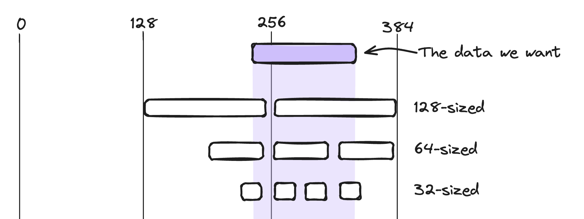
Like all of reality, GPU programming is details all the way down. Another detail is that memory loads come in a handful of preset sizes, from 32 to 512 bytes. They read contiguous memory from the memory bank, as if the data is in slots that must be read all at once.

Say we’re loading data from the memory addresses 230 to 330. Because these addresses are not aligned to the sizes of the memory loads, this would leave at least 32 bytes transferred but not actually used.³

A good way to shoot oneself in the foot is by scrambling up the data in memory so that the GPU has to load in unused data and prematurely saturate your memory bandwidth. As a consequence, a healthy mysticism is to round up sizes of data to the nearest power of 2, even if the extra computation is wasted,  because the memory loads and compiler-level optimizations can often be much more efficient⁴.

Multiprocessors

So far, we have a picture of GPUs where, once data is loaded into the GPU, all the threads can access it at the same time. In such a world, all of the threads would have to be doing the same thing at once. We couldn’t run multiple programs, nor have any of the computation go faster than the rest, resulting in a very slow and limited GPU.

To fix this, 32 threads are bunched into warps, in which all threads execute simultaneously in lockstep. But then we can run warps independently, and schedule them in and out of execution. We do this on multiprocessors, which get their own shared memory that warps can access. Data is transferred there from global memory, a much larger store for the entire GPU that all threads can access.

Memory Hierarchy

We have covered global and shared memory. What other kinds of memory are there?

Memory moves from cheap and slow, to expensive and fast. And as it moves to expensive and fast, the memory bandwidth also increases, by about 10x each level.

To get a sense of scale, let’s look at a computer set up for modern ML workloads⁵.

1. 60gb of RAM - this can store a small-to-medium sized model comfortably. Maybe it stores a small model, like Llama 2 7B, which only weighs 30gb.
2. 3gb of global memory on a V100 GPU. Already, we can expect our setup to spend a lot of time transferring weights from the host to the global memory, since the GPU can’t fit the entire model.
3. 96kb of shared memory in a multiprocessor, and that’s all we get to work with in the kernels we write. This is where data is transferred for our operation, like a matmul, to happen.
4. 1kb of registers allocated per thread, which are tiny stores of data inside the compute units. This can be thread-specific information for a program, so that threads can store private information, like a sum counter, or some variables.

We could even zoom out and think about how the data got to the computer’s RAM in the first place. Presumably it was from the computer’s storage, but was it solid state, or a hard disk, which is even slower and cheaper? Was it originally transferred from the network, and was it from a computer nearby in the data center, or was it far away?

Any minor computation triggers a cascade of data transfers in and out of the place where the computation is performed.

The Great Memory Stagnation

One of the unfortunate surprises of GPU manufacturing is that memory seems hard to scale - even harder than transistors are. ⁶ We focus so much on memory management (instead of just “getting more memory”) because memory is already about half the manufacturing cost⁷ of modern GPUs.

Because modern AI is bottlenecked by memory bandwidth, optimizations usually fall into one of a handful of categories:

• Finding ways to combine multiple operations into one (operator fusion)
• Splitting the model up into pieces that each fit on their own GPU, so that we don’t have to load the weights in and out of memory (pipeline parallelism)
• Doing more work with weights when they’re there, so as to amortize the time it took to load them in (speculative decoding, batch inference, and others)

This intricate memory hierarchy serves an important purpose in making GPU programs fast and efficient. Now that we know, we’re better equipped to wield its powers, including optimizing our silly little local models, at least until Transformer ASICs come out and totally crush us. Thankfully, that can be a story for a later day.

Thanks to Sophia Wisdom and Tom McCarthy for reviewing a draft of this post.